Importing Seahorse rates data
The read_data function imports a list of Wave excel export file(s),
meaning it will import all .xlsx files from a common
directory. With that, the user should organize the file(s) they wish to
analyze in a single directory (folder). This directory can also contain
the normalization CSV file (see Normalization). An easy way to get such a list
is to put all your data in a directory and list its contents. For
example, if your data is in a directory called “seahorse_data”:
rep_list <- list.files("seahorse_data", pattern = "*.xlsx", full.names = TRUE)In this vignette we use the package’s internal datasets:
rep_list <- system.file("extdata", package = "ceas") |>
  list.files(pattern = "*.xlsx", full.names = TRUE)
raw_data <- readxl::read_excel(rep_list[1], sheet = 2)
knitr::kable(head(raw_data))| Measurement | Well | Group | Time | OCR | ECAR | PER |
|---|---|---|---|---|---|---|
| 1 | A01 | Background | 1.304765 | 0.0000 | 0.00000 | 0.0000 |
| 1 | A02 | Group_1 MITO | 1.304765 | 305.2426 | 30.64529 | 334.4771 |
| 1 | A03 | Group_1 MITO | 1.304765 | 307.9862 | 33.27668 | 358.4754 |
| 1 | A04 | Group_2 MITO | 1.304765 | 339.3399 | 49.17751 | 503.4910 |
| 1 | A05 | Group_2 MITO | 1.304765 | 321.9398 | 47.94602 | 492.2597 |
| 1 | A06 | Group_2 MITO | 1.304765 | 323.7962 | 46.84232 | 482.1940 |
The data requires the following columns: Measurement, Well, Group,
Time, OCR, ECAR, PER. The Group column needs to be in the
format biological_group<delimiter>Assay_type (with
<space> as the default delimiter) as shown above.
Upon reading with read_data, the Group column
is split into two at the delimiter character and used to populate the
group and assay columns. This output format
can be set in the Seahorse machine before starting the experiment. The
user can choose to either
name their wells according to the ceas format on the Wave software or
manually rename each Group in the Wave excel output before importing via
read_data.If you already have the data, this column will have to be converted to this format to work with ceas.
| Measurement | Well | Time | OCR | ECAR | PER | exp_group | assay_type | replicate |
|---|---|---|---|---|---|---|---|---|
| 1 | A01 | 1.304765 | 0.0000 | 0.00000 | 0.0000 | Background | NA | 1 |
| 1 | A02 | 1.304765 | 305.2426 | 30.64529 | 334.4771 | Group_1 | MITO | 1 |
| 1 | A03 | 1.304765 | 307.9862 | 33.27668 | 358.4754 | Group_1 | MITO | 1 |
| 1 | A04 | 1.304765 | 339.3399 | 49.17751 | 503.4910 | Group_2 | MITO | 1 |
| 1 | A05 | 1.304765 | 321.9398 | 47.94602 | 492.2597 | Group_2 | MITO | 1 |
| 1 | A06 | 1.304765 | 323.7962 | 46.84232 | 482.1940 | Group_2 | MITO | 1 |
Normalization
There are two types of normalization involved in Seahorse data analysis. The first type of normalization is background normalization, which is typically performed within in the Seahorse Wave software. If the Seahorse data has been background normalized, the “Background” wells should have OCR and ECAR values of 0. ceas will flag the user with a warning if the “Background” OCR and ECAR values are not 0 (see first row of the table above).
The second type of normalization is sample normalization, which can be performed using ceas. Example sample normalization measures include cell count per well and \(\mu\)g of protein per well. Sample normalization using ceas requires an additional CSV file containing two columns:
"exp_group"or"well"experimental measure values (e.g. cell counts) in this format:
norm_csv <- system.file("extdata", package = "ceas") |>
  list.files(pattern = "norm.csv", full.names = TRUE)
norm_csv
#> [1] "/home/runner/work/_temp/Library/ceas/extdata/norm.csv"
#> [2] "/home/runner/work/_temp/Library/ceas/extdata/well_norm.csv"
exp_group_norm <- norm_csv[1]
well_norm <- norm_csv[2]

read.csv(exp_group_norm) |>
knitr::kable(caption = "For normalizing by experimental group")| exp_group | measure |
|---|---|
| Group_1 | 30000 |
| Group_2 | 30000 |
| Group_3 | 5000 |
| Group_4 | 5000 |
| Well | measure |
|---|---|
| A01 | 0 |
| A02 | 5000 |
| A03 | 5500 |
| A04 | 5300 |
| A05 | 4500 |
| A06 | 5900 |
For sample normalization ceas can use one of two normalizing
methods according to the provided norm_method argument:
"self": for each experimental group or well, the rows of the Seahorse data are divided by the correspondingmeasurevalue. Each OCR, ECAR, and PER value is divided by the measure it”self”. OCR and ECAR values are divided by the corresponding raw value in the “measure” column. This can be thought of as an intra-well/experimental group normalization. Each normalized value is then interpreted as pmol/min per cell or pmol/min per g of protein."minimum": When set to"minimum", each OCR, ECAR, and PER value is normalized by the minimum value in thenorm_csv“measure” column. In this method, every “measure” column’s value in the provided CSV file is divided by the lowest of the “measure” values to get a normalization factor for each well or experimental group. The OCR, ECAR, and PER values in each well or experimental group are divided by their corresponding normalization factors. Compared to"self", this can be thought of as an inter-well/experimental group normalization based on the lowest"measure". The results may be interpreted as pmol/min per minimum of the group cell count or g of protein.
Your normalization CSV file path may be passed into
read_data() using the norm argument along with
norm_column with either "exp_group" or
"well" and norm_method as either
"self" or "minimum".
Note: it is important to minimize sample variability during your Seahorse experiment.
read_data(
    rep_list,
    norm = exp_group_norm,
    norm_column = "exp_group",
    norm_method = "self"
) |> head() |> knitr::kable()| Measurement | Well | Time | OCR | ECAR | PER | exp_group | assay_type | replicate |
|---|---|---|---|---|---|---|---|---|
| 1 | A01 | 1.304765 | 0.0000000 | 0.0000000 | 0.0000000 | Background | NA | 1 |
| 1 | A02 | 1.304765 | 0.0101748 | 0.0010215 | 0.0111492 | Group_1 | MITO | 1 |
| 1 | A03 | 1.304765 | 0.0102662 | 0.0011092 | 0.0119492 | Group_1 | MITO | 1 |
| 1 | A04 | 1.304765 | 0.0113113 | 0.0016393 | 0.0167830 | Group_2 | MITO | 1 |
| 1 | A05 | 1.304765 | 0.0107313 | 0.0015982 | 0.0164087 | Group_2 | MITO | 1 |
| 1 | A06 | 1.304765 | 0.0107932 | 0.0015614 | 0.0160731 | Group_2 | MITO | 1 |
Calculating energetics
Partitioning data
Note:
When we use the term ‘max’ in the package documentation we mean the
maximal experimental OCR and ECAR values rather than absolute biological
maximums.
The energetics calculation workflow involves partitioning the data into its time point and assay intervals.
partitioned_data <- partition_data(seahorse_rates)Alternative data formats
The default partition_data() parameters are set to
analyze (1) Mito Stress Test and (2) Glycolysis Stress Test assays run
in parallel in the same experiment. The assay_types list
parameter can be modified to account for alternative experiments
(e.g. just a Mito Stress Test assay).
partitioned_data <- partition_data(
  seahorse_rates,
  assay_types = list(
    basal = "MITO",
    uncoupled = "MITO",
    maxresp = "MITO",
    nonmito = "MITO",
    no_glucose_glyc = "GLYCO",
    glucose_glyc = "GLYCO",
    max_glyc = "GLYCO"
  ),
  basal_tp = 3,
  uncoupled_tp = 6,
  maxresp_tp = 8,
  nonmito_tp = 12,
  no_glucose_glyc_tp = 3,
  glucose_glyc_tp = 6,
  max_glyc_tp = 8
)
partitioned_data <- partition_data(
  seahorse_rates,
  assay_types = list(
    basal = "RefAssay",
    uncoupled = "RefAssay",
    maxresp = NA,
    nonmito = "RefAssay",
    no_glucose_glyc = "RefAssay",
    glucose_glyc = "RefAssay",
    max_glyc = NA
  ),
  basal_tp = 5,
  uncoupled_tp = 10,
  nonmito_tp = 12,
  maxresp = NA,
  no_glucose_glyc_tp = 1,
  glucose_glyc_tp = 5,
  max_glyc = NA
)
partitioned_data <- partition_data(
  seahorse_rates,
  assay_types = list(
    basal = "MITO",
    uncoupled = "MITO",
    maxresp = "MITO",
    nonmito = "MITO",
    no_glucose_glyc = NA,
    glucose_glyc = "MITO",
    max_glyc = NA
  ),
  basal_tp = 3,
  uncoupled_tp = 6,
  maxresp_tp = 8,
  nonmito_tp = 12,
  no_glucose_glyc_tp = NA,
  glucose_glyc_tp = 3,
  max_glyc_tp = NA
)
partitioned_data <- partition_data(
seahorse_rates,
assay_types = list(
basal = "RCR",
uncoupled = "RCR",
maxresp = "RCR,"
nonmito = "RCR",
no_glucose_glyc = NA,
glucose_glyc = "GC",
max_glyc = "GC"
),
basal_tp = 3,
uncoupled_tp = 6,
maxresp_tp = 8,
nonmito_tp = 12,
no_glucose_glyc = NA,
glucose_glyc_tp = 3,
max_glyc_tp = 9
)Note that the time point parameters (maxresp_tp and
no_glucose_glyc_tp) also need to be changed
accordingly.
The get_energetics function requires pH, pK\(_a\) and buffer values.
energetics <- get_energetics(partitioned_data, ph = 7.4, pka = 6.093, buffer = 0.10)For more information on the calculations see the article on ATP calculations.
Plotting
Bioenergetic scope plot
The bioscope_plot function plots a 2D representation of
group “bioenergetic scope.” Bioenergetic scope describes the theoretical
energetic space in which a matrix operates. The bioenergetic scope
coordinates are JATP from OXPHOS on the y-axis and JATP from glycolysis
on the x-axis. The points represent mean basal and/or max JATP from
OXPHOS and glycolysis and the vertical and horizontal lines represent
the standard deviation or confidence interval of JATP from OXPHOS or
glycolysis, respectively.
bioscope <- bioscope_plot(
  energetics,
  model = "ols",
  sep_reps = FALSE
)
bioscope
#> Ignoring unknown labels:
#> • linetype : "Replicate"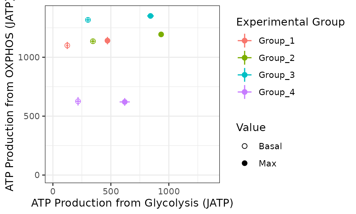
Bioenergetic scope with replicates combined
bioscope_plot(energetics, sep_reps = FALSE, model = "mixed")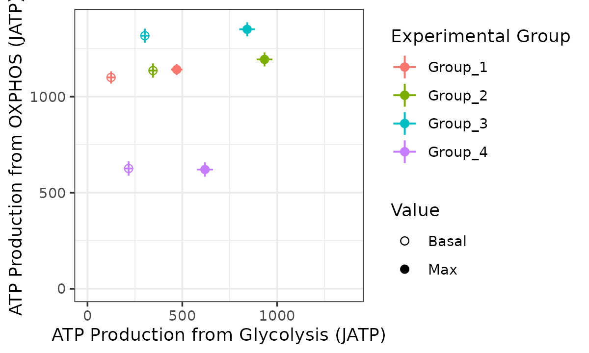
Bioenergetic scope based on a mixed-effects model with replicates as random effect
bioscope_plot(energetics, sep_reps = TRUE, model = "ols")
#> Ignoring unknown labels:
#> • linetype : "Replicate"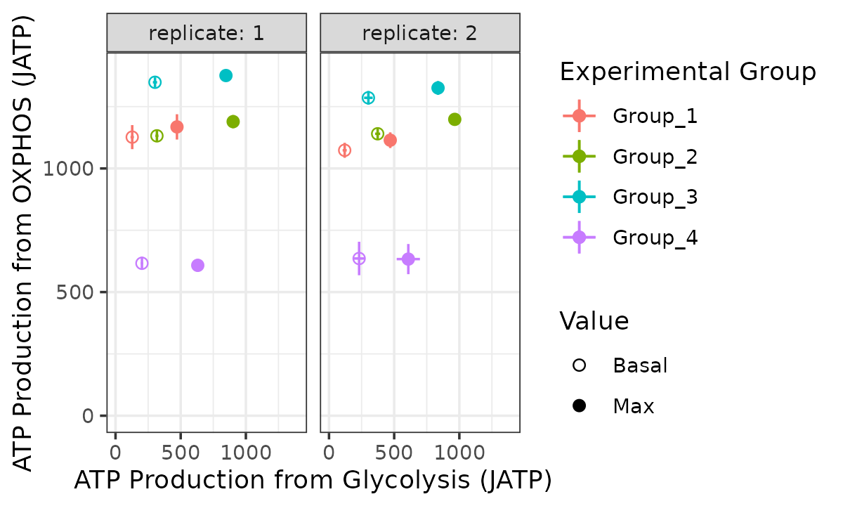
Bioenergetic scope with replicates separated
Rate plots
The rate_plot function provides an overview of OCR or
ECAR for each assay type over time, which enables cross-group energetic
comparisons before and after the addition of energetic-modulating
compounds. The rate_plot line represents mean group OCR or
ECAR over the sequential measurements (x-axis) and the shaded variance
region represents standard deviation or specified confidence
interval.
Oxygen consumption rate (OCR)
ocr <- rate_plot(
  seahorse_rates,
  measure = "OCR",
  assay = "MITO",
  model = "ols",
  sep_reps = FALSE
)
ocr
#> Ignoring unknown labels:
#> • linetype : "Replicate"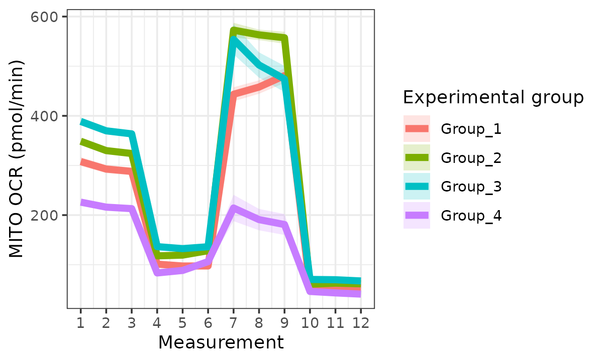
OCR with replicates combined
rate_plot(
  seahorse_rates,
  measure = "OCR",
  assay = "MITO",
  model = "mixed",
  sep_reps = FALSE
)
#> boundary (singular) fit: see help('isSingular')
#> boundary (singular) fit: see help('isSingular')
#> Ignoring unknown labels:
#> • linetype : "Replicate"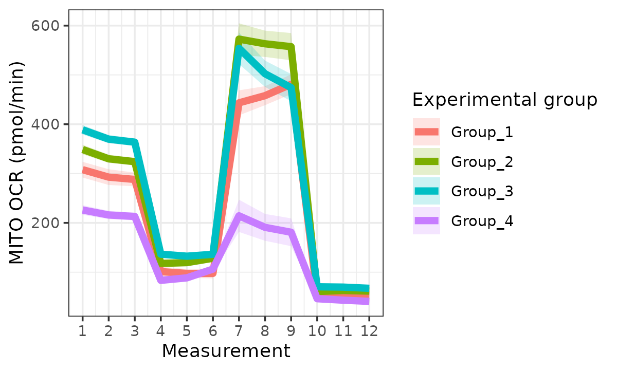
OCR based on mixed-effects model
rate_plot(
  seahorse_rates,
  measure = "OCR",
  assay = "MITO",
  model = "ols",
  sep_reps = TRUE,
  linewidth = 1
)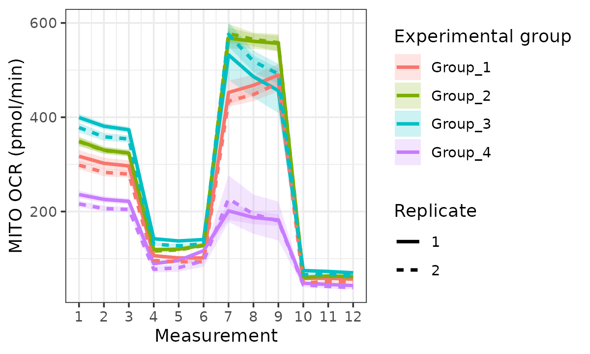
OCR with replicates separated
Extracellular Acidification Rate (ECAR)
ecar <- rate_plot(
  seahorse_rates,
  measure = "ECAR",
  assay = "GLYCO",
  model = "ols",
  sep_reps = FALSE
)
ecar
#> Ignoring unknown labels:
#> • linetype : "Replicate"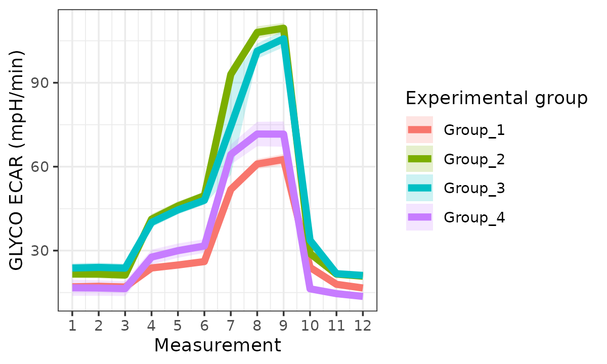
ECAR with replicates combined
rate_plot(
  seahorse_rates,
  measure = "ECAR",
  assay = "GLYCO",
  model = "mixed",
  sep_reps = FALSE
)
#> boundary (singular) fit: see help('isSingular')
#> boundary (singular) fit: see help('isSingular')
#> Ignoring unknown labels:
#> • linetype : "Replicate"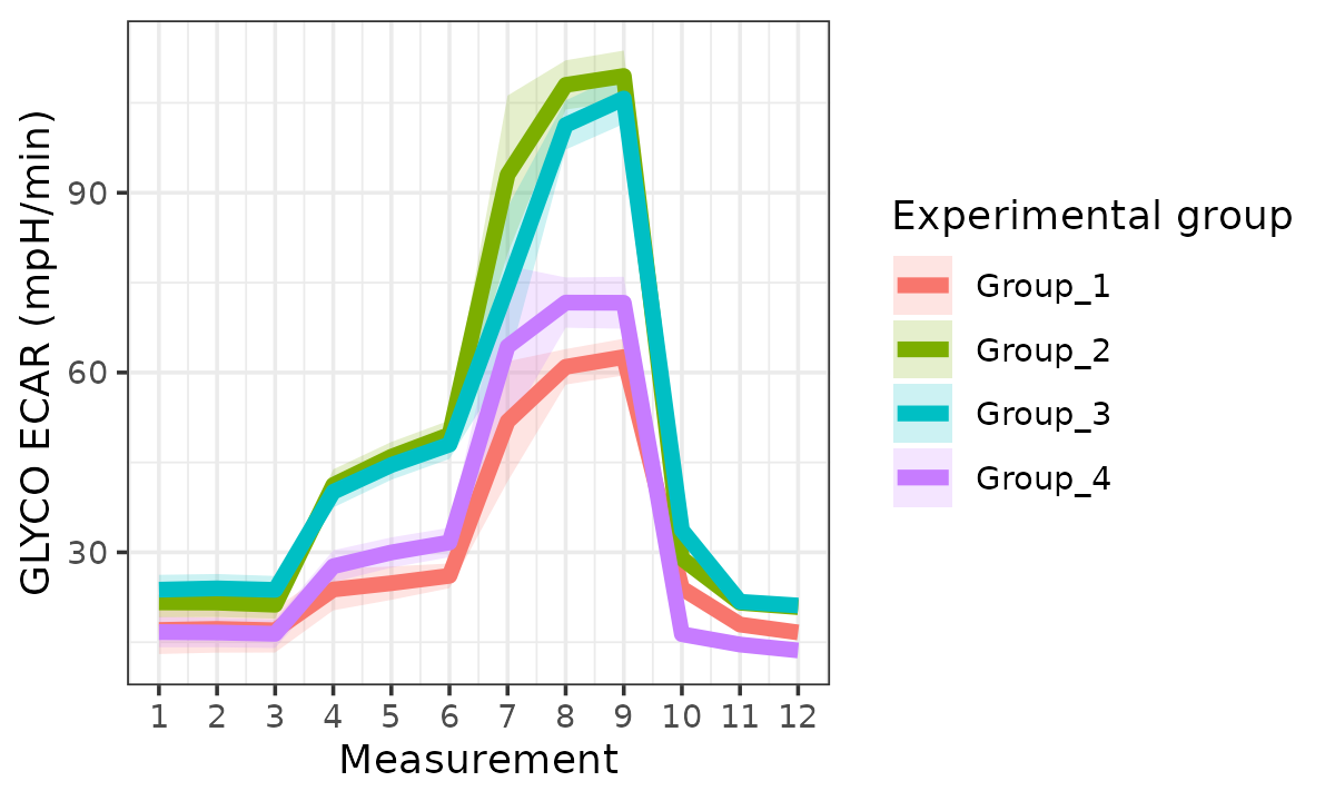
ECAR based on mixed-effects model
rate_plot(
  seahorse_rates,
  measure = "ECAR",
  assay = "GLYCO",
  model = "ols",
  sep_reps = TRUE,
  linewidth = 1

)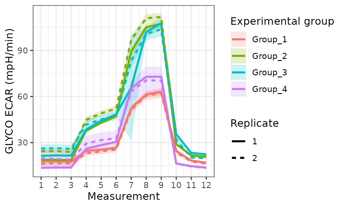
ECAR with replicates separated
ATP plots
The atp_plot function plots group JATP values, which
enables cross-group OXPHOS and glycolytic JATP comparisons at basal and
max conditions. The atp_plot symbols represent the mean
basal or max JATP from OXPHOS or glycolysis, and the crossbar boundaries
represent the standard deviation or confidence interval JATP
variance.
basal_glyc <- atp_plot(
  energetics,
  basal_vs_max = "basal",
  glyc_vs_resp = "glyc",
  sep_reps = FALSE
)
basal_glyc 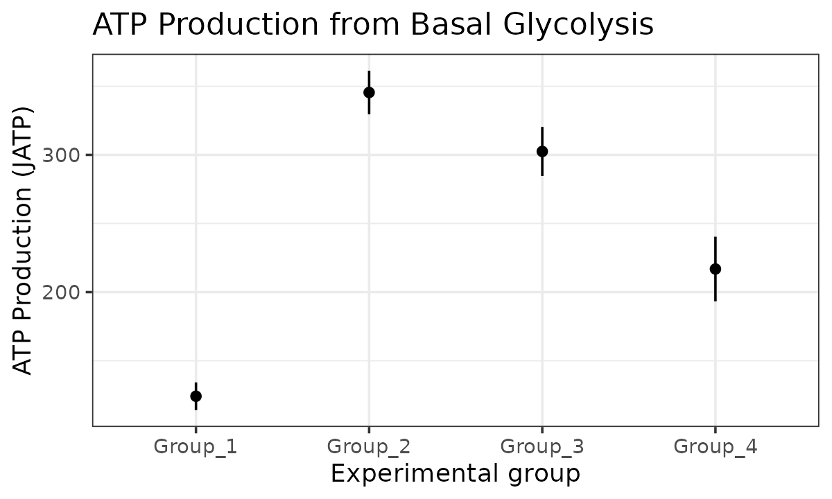
JATP from basal glycolysis with replicates combined
atp_plot(
  energetics,
  basal_vs_max = "basal",
  glyc_vs_resp = "resp",
  model = "ols",
  sep_reps = TRUE
)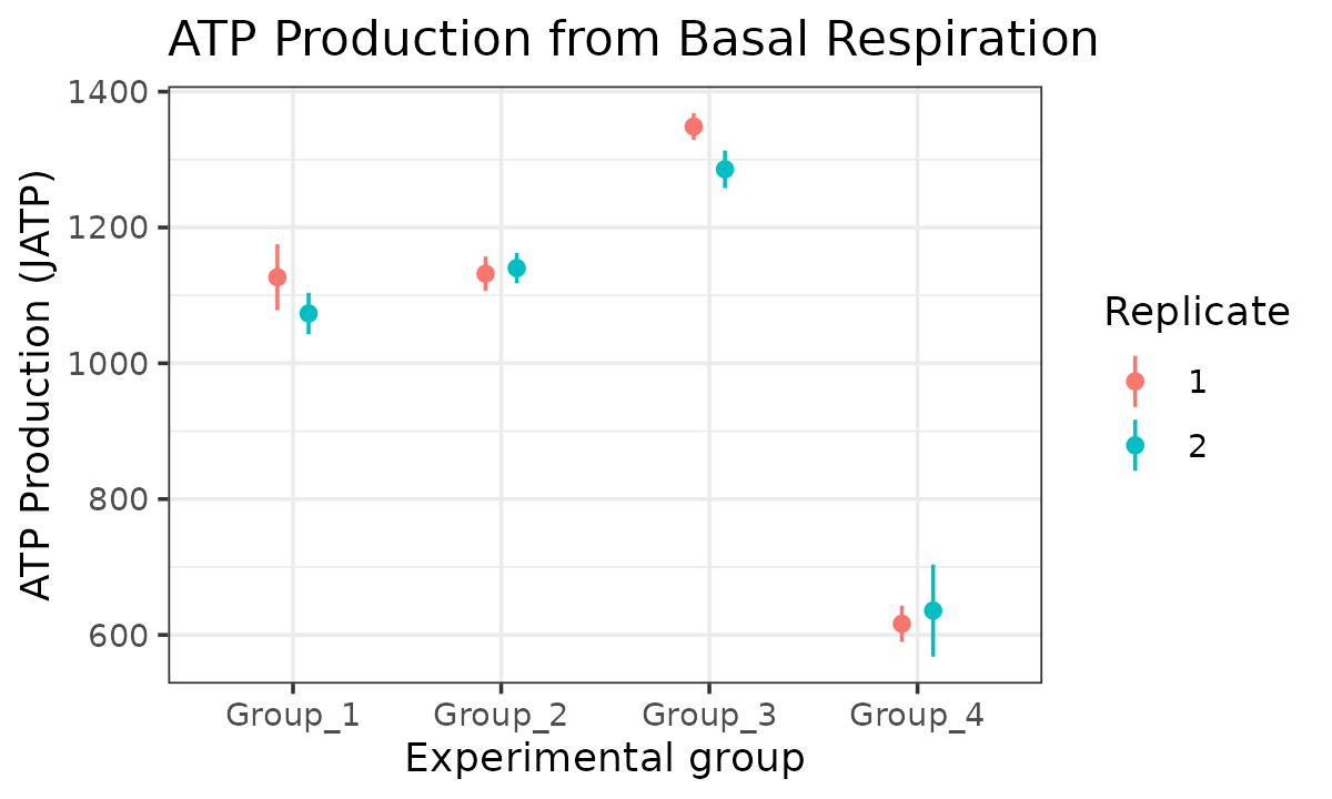
JATP from basal respiration with replicates separated
atp_plot(
  energetics,
  basal_vs_max = "max",
  glyc_vs_resp = "glyc",
  model = "mixed",
  sep_reps = FALSE
)
#> boundary (singular) fit: see help('isSingular')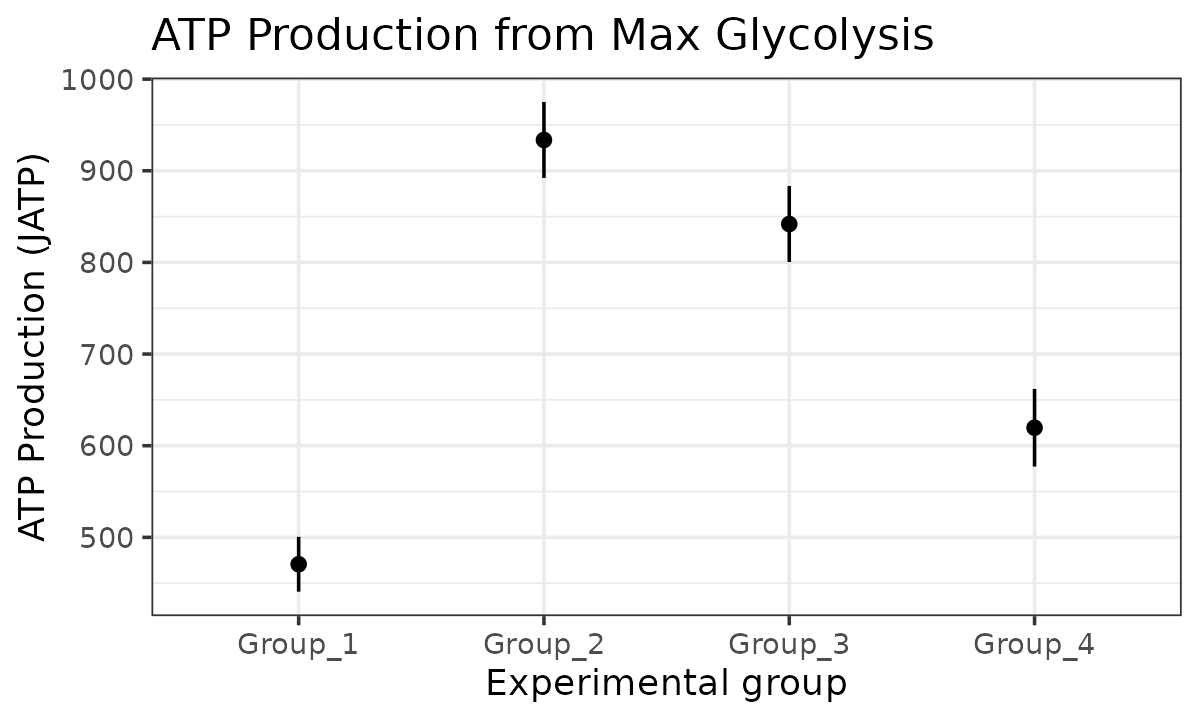
JATP from maximal glycolysis with a mixed-effects model
atp_plot(
  energetics,
  basal_vs_max = "max",
  glyc_vs_resp = "resp",
  model = "ols",
  sep_reps = TRUE
)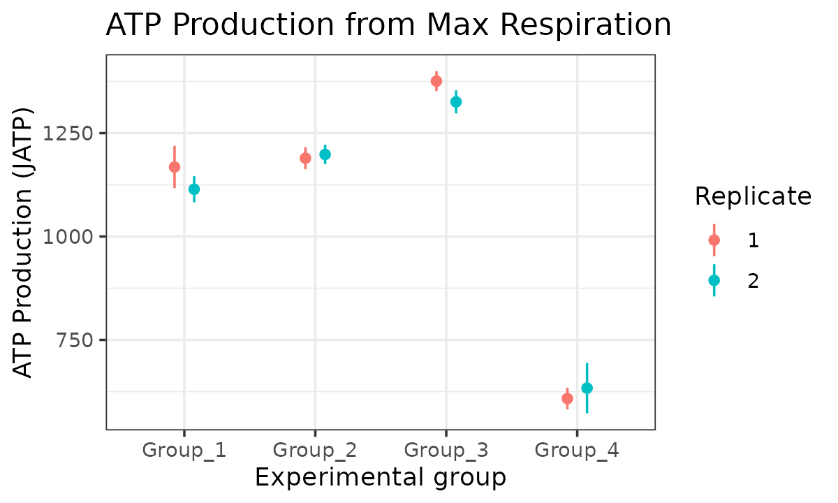
JATP from maximal respiration replicates combined
Customizing plots
CEAS is designed to work with existing ggplot2
customization functionality and doesn’t include more than shape and size
options for its plots.
For example, to change the colors used in the plot, simply make the plot and add the custom colors you’d like:
Colors
custom_colors <- c("#e36500", "#b52356", "#3cb62d", "#328fe1")
bioscope +
ggplot2::scale_color_manual(
  values = custom_colors
)
#> Ignoring unknown labels:
#> • linetype : "Replicate"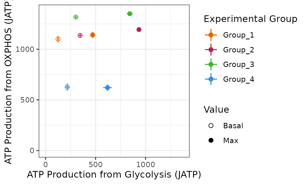
ocr +
ggplot2::scale_color_manual(
  values = custom_colors
)
#> Ignoring unknown labels:
#> • linetype : "Replicate"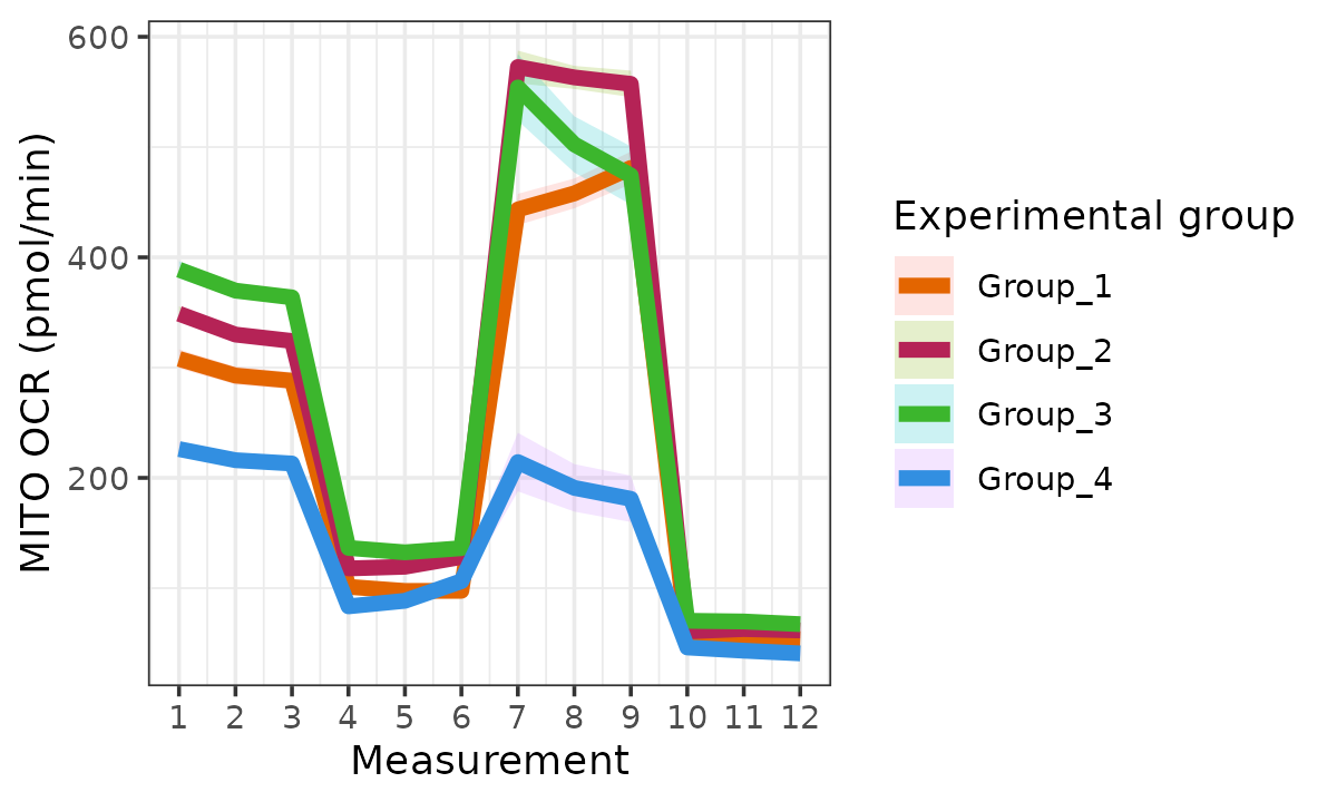
Labels
ecar +
    ggplot2::labs(x = "Time points")
#> Ignoring unknown labels:
#> • linetype : "Replicate"
basal_glyc +
    ggplot2::theme(axis.text = ggplot2::element_text(size = 20))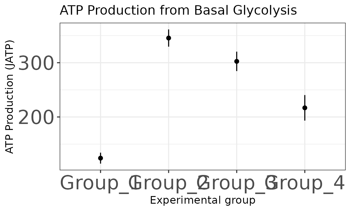
Editing functions
We are working on making the plots as customizable as possible.
However, if there are options that cannot be set in the calls to the
plotting functions or with ggplot2 functions, you can get
the code used to make the plots by running the function name without
parenthesis and modify it. Further, since every step in the ceas
workflow provides a dataset, you can run the modified function or your
own custom plotting functions on those datasets.
rate_plot
function (seahorse_rates, measure = "OCR", assay = "MITO", model = "ols",
    error_bar = "ci", conf_int = 0.95, group_label = "Experimental group",
    linewidth = 2, sep_reps = FALSE, ci_method = "Wald")
{
    stopifnot(`'measure' should be 'OCR' or 'ECAR'` = measure %in%
        c("OCR", "ECAR"))
    stopifnot(`'model' should be 'ols' or 'mixed'` = model %in%
        c("ols", "mixed"))
    stopifnot(`cannot run mixed-effects model with \`sep_reps = TRUE\`` = (model ==
        "mixed" & !sep_reps) | (model == "ols"))
    stopifnot(`'error_bar' should be 'sd' or 'ci'` = error_bar %in%
        c("sd", "ci"))
    stopifnot(`'conf_int' should be between 0 and 1` = conf_int >
        0 && conf_int < 1)
    data_cols <- c("Measurement", "Well", "OCR", "ECAR", "PER",
        "exp_group", "assay_type", "replicate")
    missing_cols <- setdiff(data_cols, colnames(seahorse_rates))
    if (length(missing_cols) != 0) {
        stop(paste0("'", missing_cols, "'", " column was not found in input data\n"))
    }
    Measurement <- NULL
    exp_group <- NULL
    lower_bound <- NULL
    upper_bound <- NULL
    multi_rep <- length(unique(seahorse_rates$replicate)) > 1
    if (!sep_reps && missing(sep_reps) && multi_rep) {
        warning(sep_reps_warning)
    }
    plot_data <- get_rate_summary(seahorse_rates, measure, assay,
        model, error_bar, conf_int, sep_reps)
    y_labels <- list(OCR = paste0(assay, " OCR (pmol/min)"),
        ECAR = paste0(assay, " ECAR (mpH/min)"))
    p <- ggplot(plot_data, aes(x = Measurement, y = mean, color = exp_group,
        group = if (sep_reps && multi_rep)
            interaction(exp_group, replicate)
        else exp_group, fill = exp_group)) + geom_ribbon(aes(ymin = lower_bound,
        ymax = upper_bound), alpha = 0.2, color = NA) + scale_x_continuous(breaks = seq(1,
        12, by = 1)) + xlab("Measurement") + ylab(y_labels[measure]) +
        labs(color = group_label, fill = group_label, linetype = "Replicate") +
        theme_bw()
    if (sep_reps && multi_rep) {
        p + geom_line(aes(linetype = replicate), linewidth = linewidth)
    }
    else {
        p + geom_line(linewidth = linewidth)
    }
}
In RStudio, you can run utils::edit to modify a
function.
edit(rate_plot)